Quickstart
ParMOO is a parallel multiobjective optimization solver that seeks to exploit simulation-based structure in objective and constraint functions.
To exploit structure, ParMOO models simulations separately from objectives and constraints. In our language:
a design variable is an input to the problem, which we can directly control;
a simulation is an expensive or time-consuming process, including real-world experimentation, which is treated as a blackbox function of the design variables and evaluated sparingly;
an objective is an algebraic function of the design variables and/or simulation outputs, which we would like to optimize; and
a constraint is an algebraic function of the design variables and/or simulation outputs, which cannot exceed a specified bound.
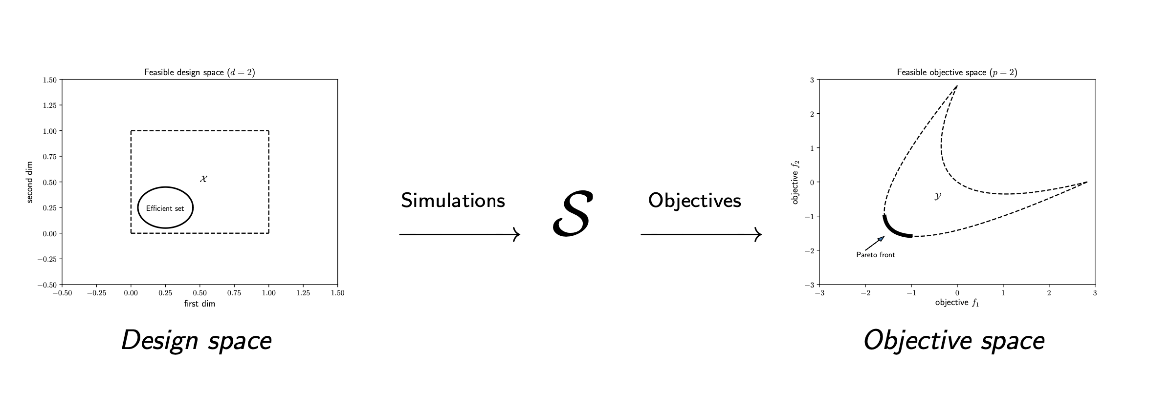
To solve a multiobjective optimization problem (MOOP), we use surrogate models of the simulation outputs, together with the algebraic definition of the objectives and constraints.
In order to achieve scalable parallelism, we use libEnsemble to distribute batches of simulation evaluations across parallel resources.
Dependencies
ParMOO has been tested on Unix/Linux and MacOS systems.
ParMOO’s base has the following dependencies:
Additional dependencies are needed to use the additional features in
parmoo.extras:
libEnsemble – for managing parallel simulation evaluations
And for using the Pareto front visualization library in parmoo.viz:
Installation
The easiest way to install ParMOO is via the Python package index, PyPI
(commonly called pip):
pip install < --user > parmoo
where the braces around < --user > indicate that the --user flag is
optional.
To install all dependencies (including libEnsemble) use:
pip install < --user > "parmoo[extras]"
Note that the full feature set for libEnsemble and kaleido may require you to separately install an MPI implementation (such as Open_MPI) and Google chrome (e.g., via kaleido_get_chrome), respectively.
You can also clone this project from our GitHub and pip install it
in-place, so that you can easily pull the latest version or checkout
the develop branch for pre-release features.
On Debian-based systems with a bash shell, this looks like:
git clone https://github.com/parmoo/parmoo
cd parmoo
pip install -e .
Alternatively, the latest release of ParMOO (including all required and
optional dependencies) can be installed from the conda-forge channel using:
conda install --channel=conda-forge parmoo
Before doing so, it is recommended to create a new conda environment using:
conda create --name channel-name
conda activate channel-name
For detailed instructions, see Advanced Installation.
Testing
Note that in order to run the unit tests, you must first install the
parmoo[extras], as described above. This may include the additional steps
such as kaleido_get_chrome.
You can install pytest with the pytest-cov plugin and flake8 using the
tests extension, then you can lint the project with flake8 and run the
unit tests for your installation using pytest. After running unit tests,
you can view the coverage report using the coverage report command.
pip install -e ".[tests]"
flake8 parmoo
pytest
coverage report
Running the regression tests and libEnsemble tests is a bit more involved and
is usually accomplished via the -l flag for the
parmoo/tests/run-tests.sh script.
To run all the linter, unit tests, regression tests, and generate the coverage report in a single command, run the script with all 4 flags set.
These tests are run regularly using GitHub Actions.
Basic Usage
ParMOO uses numpy and jax in an object-oriented design, based around the
MOOP class.
Before getting started, note that jax runs in single (32-bit) precision by default. To run in double precision, the following code is needed at startup:
import jax
jax.config.update("jax_enable_x64", True)
This will be done automatically when importing certain modules in ParMOO, which are only compatible with double precision. However, in many use cases, 32-bit precision may be enough and provides substantial speedup in iteration tasks.
Once the precision is set, to get started,
create a MOOP object, using the
constructor.
from parmoo import MOOP
from parmoo.optimizers import GlobalSurrogate_PS

my_moop = MOOP(GlobalSurrogate_PS)
To summarize the framework, in each iteration ParMOO models each simulation
using a computationally cheap surrogate, then solves one or more scalarizations
of the objectives, which are specified by acquisition functions.
Read more about this framework at our Learn About MOOPs page.
In the above example,
optimizers.GlobalSurrogate_PS
is the class of optimizers
that the my_moop object will use to solve the scalarized surrogate
problems.
Next, add design variables to the problem as follows using the
MOOP.addDesign(*args) method.
In this example, we define one continuous and one categorical design variable.
Other options include integer, custom, and raw (using raw variables is not
recommended except for expert users).
# Add a single continuous design variable in the range [0.0, 1.0]
my_moop.addDesign({'name': "x1", # optional, name
                   'des_type': "continuous", # optional, type of variable
                   'lb': 0.0, # required, lower bound
                   'ub': 1.0, # required, upper bound
                   'tol': 1.0e-8 # optional tolerance
                  })
# Add a second categorical design variable with 3 levels
my_moop.addDesign({'name': "x2", # optional, name
                   'des_type': "categorical", # required, type of variable
                   'levels': [-1, 1] # required, list of category labels
                  })
Next, add simulations to the problem as follows using the
MOOP.addSimulation(*args) method.
In this example, we define a toy simulation sim_func(x).
import numpy as np
from parmoo.searches import LatinHypercube
from parmoo.surrogates import GaussRBF

# Define a toy simulation for the problem, whose outputs are quadratic
def sim_func(x):
   sx = np.array([(x["x1"] - 0.2) ** 2, (x["x1"] - 0.8) ** 2])
   if x["x2"] != 1: sx += 99.
   return sx
# Add the simulation to the problem
my_moop.addSimulation({'name': "MySim", # Optional name for this simulation
                       'm': 2, # This simulation has 2 outputs
                       'sim_func': sim_func, # Our sample sim from above
                       'search': LatinHypercube, # Use a LHS search
                       'surrogate': GaussRBF, # Use a Gaussian RBF surrogate
                       'hyperparams': {}, # Hyperparams passed to internals
                       'sim_db': { # Optional dict of precomputed points
                                  'search_budget': 10 # Set search budget
                                 },
                      })
Now we can add objectives and constraints using
MOOP.addObjective(*args) and
MOOP.addConstraint(*args).
In this example, there are 2 objectives (each corresponding to a single
simulation output) and one constraint.
# First objective just returns the first simulation output
def f1(x, s): return s["MySim"][0]
my_moop.addObjective({'name': "f1", 'obj_func': f1})
# Second objective just returns the second simulation output
def f2(x, s): return s["MySim"][1]
my_moop.addObjective({'name': "f2", 'obj_func': f2})
# Add a single constraint, that x[0] >= 0.1
def c1(x, s): return 0.1 - x["x1"]
my_moop.addConstraint({'name': "c1", 'con_func': c1})
Finally, we must add one or more acquisition functions using
MOOP.addAcquisition(*args).
These are used to scalarize the surrogate problems.
The number of acquisition functions
typically determines the number of simulation evaluations per batch.
This is useful to know if you are using a parallel solver.
from parmoo.acquisitions import RandomConstraint

# Add 3 acquisition functions
for i in range(3):
   my_moop.addAcquisition({'acquisition': RandomConstraint,
                           'hyperparams': {}})
Finally, the MOOP is solved using the
MOOP.solve(budget) method, and the
results can be viewed using
MOOP.getPF().
import pandas as pd

my_moop.solve(5) # Solve with 5 iterations of ParMOO algorithm
results = my_moop.getPF(format="pandas") # Extract the results as pandas df
After executing the above block of code, the results variable points to
a pandas dataframe, each of whose rows corresponds to a nondominated
objective value in the my_moop object’s final database.
You can reference individual columns in the results array by using the
name keys that were assigned during my_moop’s construction, or
plot the results by using the viz library.
Congratulations, you now know enough to get started solving MOOPs!
Minimal Working Example
Putting it all together, we get the following minimal working example.
import numpy as np
from parmoo import MOOP
from parmoo.searches import LatinHypercube
from parmoo.surrogates import GaussRBF
from parmoo.acquisitions import RandomConstraint
from parmoo.optimizers import GlobalSurrogate_PS

# Fix the random seed for reproducibility using the np_random_gen hyperparams
my_moop = MOOP(GlobalSurrogate_PS, hyperparams={'np_random_gen': 0})

my_moop.addDesign({'name': "x1",
                   'des_type': "continuous",
                   'lb': 0.0, 'ub': 1.0})
# Note: the 'levels' key can contain a list of strings, but jax can only jit
# numeric types, so integer level IDs are strongly recommended
my_moop.addDesign({'name': "x2", 'des_type': "categorical",
                   'levels': [-1, 1]})

def sim_func(x):
   sx = np.array([(x["x1"] - 0.2) ** 2, (x["x1"] - 0.8) ** 2])
   ## The following 2 lines are equivalent, but jax cannot jit if statements.
   ## Uncomment below to see the difference in execution speed from jit
   # if x["x2"] != 1: sx += 99.
   sx += 99. - 99. * (x["x2"] == 1)
   return sx

my_moop.addSimulation({'name': "MySim",
                       'm': 2,
                       'sim_func': sim_func,
                       'search': LatinHypercube,
                       'surrogate': GaussRBF,
                       'hyperparams': {'search_budget': 20}})

def f1(x, s): return s["MySim"][0]
def f2(x, s): return s["MySim"][1]
my_moop.addObjective({'name': "f1", 'obj_func': f1})
my_moop.addObjective({'name': "f2", 'obj_func': f2})

def c1(x, s): return 0.1 - x["x1"]
my_moop.addConstraint({'name': "c1", 'constraint': c1})

for i in range(3):
   my_moop.addAcquisition({'acquisition': RandomConstraint,
                           'hyperparams': {}})

my_moop.solve(5)
results = my_moop.getPF(format="pandas")

# Display solution
print(results)

# Plot results -- must have extra viz dependencies installed
from parmoo.viz import scatter
# The optional arg `output` exports directly to jpeg instead of interactive mode
scatter(my_moop, output="jpeg")
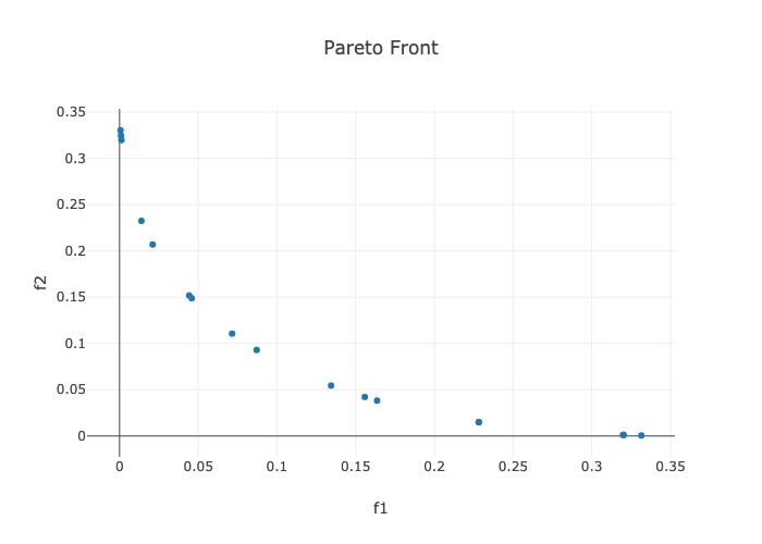
The above code saves all (approximate) Pareto optimal solutions in the
results variable, and prints the results variable to the standard
output:
          x1  x2        f1        f2        c1
0   0.775789   1  0.331533  0.000586 -0.675789
1   0.765908   1  0.320252  0.001162 -0.665908
2   0.765517   1  0.319810  0.001189 -0.665517
3   0.677822   1  0.228314  0.014927 -0.577822
4   0.677627   1  0.228127  0.014975 -0.577627
5   0.604457   1  0.163585  0.038237 -0.504457
6   0.594717   1  0.155801  0.042141 -0.494717
7   0.566581   1  0.134382  0.054484 -0.466581
8   0.495124   1  0.087098  0.092949 -0.395124
9   0.467398   1  0.071502  0.110624 -0.367398
10  0.414142   1  0.045857  0.148886 -0.314142
11  0.410334   1  0.044240  0.151840 -0.310334
12  0.345129   1  0.021062  0.206908 -0.245129
13  0.317883   1  0.013896  0.232437 -0.217883
14  0.234523   1  0.001192  0.319764 -0.134523
15  0.230129   1  0.000908  0.324753 -0.130129
16  0.225272   1  0.000639  0.330312 -0.125272
And produces the following figure of the Pareto points:
Next Steps
If you want to take advantage of all that ParMOO has to offer, please see Writing a ParMOO Script.
If you would like more information on multiobjective optimization terminology and ParMOO’s methodology, see the Learn About MOOPs page.
For a full list of basic usage tutorials, see More Tutorials.
To start solving MOOPs on parallel hardware, install libEnsemble and see the libEnsemble tutorial.
See some of our pre-built solvers in the parmoo_solver_farm.
To interactively explore your solutions, install its extra dependencies and use our built-in viz tool.
For more advice, consult our FAQs.
Resources
To seek support or report issues, e-mail:
parmoo@lbl.gov
Our full documentation is hosted on:
Please read our LICENSE and CONTRIBUTING files.