Basic Tutorials
This is a collection of all tutorials demonstrating basic ParMOO functionality (collected from throughout the ParMOO User Guide).
Quickstart Demo
This is a basic example (see quickstart.py) of how to build and solve a MOOP with ParMOO, taken from the Quickstart guide.
import numpy as np
from parmoo import MOOP
from parmoo.searches import LatinHypercube
from parmoo.surrogates import GaussRBF
from parmoo.acquisitions import RandomConstraint
from parmoo.optimizers import GlobalSurrogate_PS

# Fix the random seed for reproducibility using the np_random_gen hyperparams
my_moop = MOOP(GlobalSurrogate_PS, hyperparams={'np_random_gen': 0})

my_moop.addDesign({'name': "x1",
                   'des_type': "continuous",
                   'lb': 0.0, 'ub': 1.0})
# Note: the 'levels' key can contain a list of strings, but jax can only jit
# numeric types, so integer level IDs are strongly recommended
my_moop.addDesign({'name': "x2", 'des_type': "categorical",
                   'levels': [-1, 1]})

def sim_func(x):
   sx = np.array([(x["x1"] - 0.2) ** 2, (x["x1"] - 0.8) ** 2])
   ## The following 2 lines are equivalent, but jax cannot jit if statements.
   ## Uncomment below to see the difference in execution speed from jit
   # if x["x2"] != 1: sx += 99.
   sx += 99. - 99. * (x["x2"] == 1)
   return sx

my_moop.addSimulation({'name': "MySim",
                       'm': 2,
                       'sim_func': sim_func,
                       'search': LatinHypercube,
                       'surrogate': GaussRBF,
                       'hyperparams': {'search_budget': 20}})

def f1(x, s): return s["MySim"][0]
def f2(x, s): return s["MySim"][1]
my_moop.addObjective({'name': "f1", 'obj_func': f1})
my_moop.addObjective({'name': "f2", 'obj_func': f2})

def c1(x, s): return 0.1 - x["x1"]
my_moop.addConstraint({'name': "c1", 'constraint': c1})

for i in range(3):
   my_moop.addAcquisition({'acquisition': RandomConstraint,
                           'hyperparams': {}})

my_moop.solve(5)
results = my_moop.getPF(format="pandas")

# Display solution
print(results)

# Plot results -- must have extra viz dependencies installed
from parmoo.viz import scatter
# The optional arg `output` exports directly to jpeg instead of interactive mode
scatter(my_moop, output="jpeg")
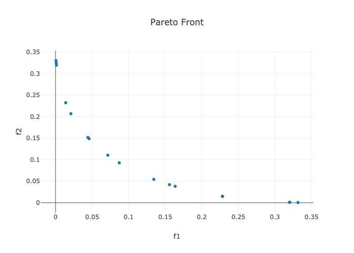
The above code saves all (approximate) Pareto optimal solutions in the
results dataframe, and prints the results dataframe to the standard
output:
          x1  x2        f1        f2        c1
0   0.775789   1  0.331533  0.000586 -0.675789
1   0.765908   1  0.320252  0.001162 -0.665908
2   0.765517   1  0.319810  0.001189 -0.665517
3   0.677822   1  0.228314  0.014927 -0.577822
4   0.677627   1  0.228127  0.014975 -0.577627
5   0.604457   1  0.163585  0.038237 -0.504457
6   0.594717   1  0.155801  0.042141 -0.494717
7   0.566581   1  0.134382  0.054484 -0.466581
8   0.495124   1  0.087098  0.092949 -0.395124
9   0.467398   1  0.071502  0.110624 -0.367398
10  0.414142   1  0.045857  0.148886 -0.314142
11  0.410334   1  0.044240  0.151840 -0.310334
12  0.345129   1  0.021062  0.206908 -0.245129
13  0.317883   1  0.013896  0.232437 -0.217883
14  0.234523   1  0.001192  0.319764 -0.134523
15  0.230129   1  0.000908  0.324753 -0.130129
16  0.225272   1  0.000639  0.330312 -0.125272
And produces the following figure of the Pareto points:
The name Key and Input/Output Types
The following named_var_ex.py code demonstrates ParMOO’s output datatypes
and proper definition of the MOOP object.
import numpy as np
from parmoo import MOOP
from parmoo.searches import LatinHypercube
from parmoo.surrogates import GaussRBF
from parmoo.optimizers import GlobalSurrogate_PS

my_moop = MOOP(GlobalSurrogate_PS)

# Define a simulation to use below
def sim_func(x):
    if x["MyCat"] == 0:
        return np.array([(x["MyDes"]) ** 2, (x["MyDes"] - 1.0) ** 2])
    else:
        return np.array([99.9, 99.9])

# Add a design variable, simulation, objective, and constraint.
# Note the 'name' keys for each
my_moop.addDesign({'name': "MyDes",
                   'des_type': "continuous",
                   'lb': 0.0, 'ub': 1.0})
my_moop.addDesign({'name': "MyCat",
                   'des_type': "categorical",
                   'levels': 2})

my_moop.addSimulation({'name': "MySim",
                       'm': 2,
                       'sim_func': sim_func,
                       'search': LatinHypercube,
                       'surrogate': GaussRBF,
                       'hyperparams': {'search_budget': 20}})

my_moop.addObjective({'name': "MyObj",
                      'obj_func': lambda x, s: sum(s["MySim"])})

my_moop.addConstraint({'name': "MyCon",
                       'constraint': lambda x, s: 0.1 - x["MyDes"]})

# Extract numpy dtypes for all of this MOOP's inputs/outputs
des_dtype = my_moop.getDesignType()
obj_dtype = my_moop.getObjectiveType()
sim_dtype = my_moop.getSimulationType()

# Display the dtypes as strings
print("Design variable type:   " + str(des_dtype))
print("Simulation output type: " + str(sim_dtype))
print("Objective type:         " + str(obj_dtype))
The above code produces the following output.
Design variable type:   [('MyDes', '<f8'), ('MyCat', '<i4')]
Simulation output type: [('MySim', '<f8', (2,))]
Objective type:         [('MyObj', '<f8')]
Adding Precomputed Simulation Values
The following precomputed_data.py code demonstrates how to add a precomputed simulation output to ParMOO’s internal simulation databases.
import numpy as np
from parmoo import MOOP
from parmoo.searches import LatinHypercube
from parmoo.surrogates import GaussRBF
from parmoo.acquisitions import UniformWeights
from parmoo.optimizers import GlobalSurrogate_PS

my_moop = MOOP(GlobalSurrogate_PS)

my_moop.addDesign({'name': "x1",
                   'des_type': "continuous",
                   'lb': 0.0, 'ub': 1.0})
my_moop.addDesign({'name': "x2", 'des_type': "categorical",
                   'levels': 3})

def sim_func(x):
   if x["x2"] == 0:
      return np.array([(x["x1"] - 0.2) ** 2, (x["x1"] - 0.8) ** 2])
   else:
      return np.array([99.9, 99.9])

my_moop.addSimulation({'name': "MySim",
                       'm': 2,
                       'sim_func': sim_func,
                       'search': LatinHypercube,
                       'surrogate': GaussRBF,
                       'hyperparams': {'search_budget': 20}})

my_moop.addObjective({'name': "f1", 'obj_func': lambda x, s: s["MySim"][0]})
my_moop.addObjective({'name': "f2", 'obj_func': lambda x, s: s["MySim"][1]})

my_moop.addAcquisition({'acquisition': UniformWeights})

# This step is needed to finalize the MOOP definition. If you are using the
# solve command it is done automatically, but it must be done manually before
# any pre-existing data can be added.
my_moop.compile()

# Precompute one simulation value for demo
des_val = np.zeros(1, dtype=[("x1", float), ("x2", int)])[0]
sim_val = sim_func(des_val)

# Add the precomputed simulation value from above
my_moop.updateSimDb(des_val, sim_val, "MySim")

# Get and display initial database
sim_db = my_moop.getSimulationData()
print(sim_db)
The above code produces the following output.
{'MySim': array([(0., 0, [0.04, 0.64])],
      dtype=[('x1', '<f8'), ('x2', '<i4'), ('out', '<f8', (2,))])}
Logging and Checkpointing
When solving a large or expensive problem, logging and checkpointing are recommended. The following code snippet shows how to solve the same problem from the Quickstart example, but with logging and checkpointing turned on. Then, another MOOP is created by reloading from the checkpoint file, and run for 1 extra iteration, in order to demonstrate how to reload from a saved checkpoint file.
Note how the lambda functions from Quickstart example have been explicitly defined below. This is because ParMOO reloads functions by name, which means that it does not support checkpointing for lambda functions and any named function must be defined with the same name in the global scope during reloading.
import numpy as np
from parmoo import MOOP
from parmoo.searches import LatinHypercube
from parmoo.surrogates import GaussRBF
from parmoo.acquisitions import UniformWeights
from parmoo.optimizers import GlobalSurrogate_PS
import logging

# Create a new MOOP -- fix the random seed with the hyperparams
my_moop = MOOP(GlobalSurrogate_PS, hyperparams={'np_random_gen': 0})

# Add 1 continuous and 1 categorical design variable
my_moop.addDesign({'name': "x1",
                   'des_type': "continuous",
                   'lb': 0.0, 'ub': 1.0})
my_moop.addDesign({'name': "x2", 'des_type': "categorical",
                   'levels': 3})

# Create a simulation function
def sim_func(x):
   if x["x2"] == 0:
      return np.array([(x["x1"] - 0.2) ** 2, (x["x1"] - 0.8) ** 2])
   else:
      return np.array([99.9, 99.9])

# Add the simulation function to the MOOP
my_moop.addSimulation({'name': "MySim",
                       'm': 2,
                       'sim_func': sim_func,
                       'search': LatinHypercube,
                       'surrogate': GaussRBF,
                       'hyperparams': {'search_budget': 20}})

# Define the 2 objectives as named Python functions
def obj1(x, s): return s["MySim"][0]
def obj2(x, s): return s["MySim"][1]

# Define the constraint as a function
def const(x, s): return 0.1 - x["x1"]

# Add 2 objectives
my_moop.addObjective({'name': "f1", 'obj_func': obj1})
my_moop.addObjective({'name': "f2", 'obj_func': obj2})

# Add 1 constraint
my_moop.addConstraint({'name': "c1", 'constraint': const})

# Add 3 acquisition functions (generates batches of size 3)
for i in range(3):
   my_moop.addAcquisition({'acquisition': UniformWeights,
                           'hyperparams': {}})

# Turn on logging with timestamps
logging.basicConfig(level=logging.INFO,
                    format='%(asctime)s %(levelname)-8s %(message)s',
                    datefmt='%Y-%m-%d %H:%M:%S')

# Use checkpointing without saving a separate data file (in "parmoo.moop" file)
my_moop.setCheckpoint(True, filename="parmoo")

# Solve the problem with 4 iterations
my_moop.solve(4)

# Create a new MOOP object and reload the MOOP from parmoo.moop file
new_moop = MOOP(GlobalSurrogate_PS)
new_moop.load("parmoo")

# Do another iteration
new_moop.solve(5)

# Display the solution
results = new_moop.getPF()
print(results, "\n dtype=" + str(results.dtype))
The above checkpointing.py code produces the following output.
[(0.78651355, 0, 0.34399814, 1.81884372e-04, -0.68651355)
 (0.72175941, 0, 0.27223289, 6.12158940e-03, -0.62175941)
 (0.71746254, 0, 0.26776748, 6.81243257e-03, -0.61746254)
 (0.71560707, 0, 0.26585065, 7.12216670e-03, -0.61560707)
 (0.71433754, 0, 0.2645431 , 7.33805733e-03, -0.61433754)
 (0.71033363, 0, 0.26044042, 8.04005753e-03, -0.61033363)
 (0.66769687, 0, 0.21874036, 1.75041176e-02, -0.56769687)
 (0.62648593, 0, 0.18189025, 3.01071308e-02, -0.52648593)
 (0.55285312, 0, 0.12450533, 6.10815791e-02, -0.45285312)
 (0.52941562, 0, 0.10851465, 7.32159054e-02, -0.42941562)
 (0.44156652, 0, 0.05835439, 1.28474557e-01, -0.34156652)
 (0.43785559, 0, 0.05657528, 1.31148576e-01, -0.33785559)
 (0.39723059, 0, 0.0388999 , 1.62223200e-01, -0.29723059)
 (0.34928137, 0, 0.02228493, 2.03147285e-01, -0.24928137)
 (0.32389074, 0, 0.01534892, 2.26680025e-01, -0.22389074)
 (0.30592199, 0, 0.01121947, 2.44113077e-01, -0.20592199)
 (0.29342199, 0, 0.00872767, 2.56621277e-01, -0.19342199)
 (0.28407396, 0, 0.00706843, 2.66179683e-01, -0.18407396)
 (0.24208177, 0, 0.00177088, 3.11272754e-01, -0.14208177)
 (0.22899583, 0, 0.00084076, 3.26045762e-01, -0.12899583)]
 dtype=[('x1', '<f8'), ('x2', '<i4'), ('f1', '<f8'), ('f2', '<f8'), ('c1', '<f8')]
Solving a MOOP with Derivative-Based Solvers
This example shows how to minimize two conflicting quadratic functions
of three variables (named x1, x2, and x3),
under the constraint that an additional categorical variable (x4)
must be fixed in class 0 \(^*\),
using the derivative-based solvers, such as one of the
LBFGSB solvers.
\(^*\) No, this constraint does not really affect the solution;
it is just here to demonstrate how constraints/categorical variables
are handled by derivative-based solvers.
ParMOO does not use derivative information associated with
any categorical variables, so the derivative w.r.t. x4 can be set
to any value, without affecting the outcome.
import numpy as np
from parmoo import MOOP
from parmoo.acquisitions import RandomConstraint, FixedWeights
from parmoo.searches import LatinHypercube
from parmoo.surrogates import GaussRBF
from parmoo.optimizers import GlobalSurrogate_BFGS
import logging

# Create a new MOOP with a derivative-based solver
my_moop = MOOP(GlobalSurrogate_BFGS,
               # Use the hyperparams to fix the random seed for reproducibility
               hyperparams={'np_random_gen': 0})

# Add 3 continuous variables named x1, x2, x3
for i in range(3):
    my_moop.addDesign({'name': f"x{i+1}",
                       'des_type': "continuous",
                       'lb': 0.0,
                       'ub': 1.0,
                       'des_tol': 1.0e-8})
# Add one categorical variable named x4
my_moop.addDesign({'name': "x4",
                   'des_type': "categorical",
                   'levels': 3})


def quad_sim(x):
    """ A quadratic simulation function with 2 outputs.

    Returns:
        np.ndarray: simulation value (S) with 2 outputs
         * S_1(x) = <x, x>
         * S_2(x) = <x-1, x-1>

    """

    return np.array([x["x1"] ** 2 + x["x2"] ** 2 + x["x3"] ** 2,
                     (x["x1"] - 1.0) ** 2 + (x["x2"] - 1.0) ** 2 +
                     (x["x3"] - 1.0) ** 2])


# Add the quadratic simulation to the problem
# Use a 10-point LHS experimental design and a Gaussian RBF surrogate model
my_moop.addSimulation({'name': "f_conv",
                       'm': 2,
                       'sim_func': quad_sim,
                       'search': LatinHypercube,
                       'surrogate': GaussRBF,
                       'hyperparams': {'search_budget': 10}})


# Define some objectives below -- try to avoid things that jax can't compile


def obj_f1_func(x, sim):
    """ Minimize the first output from 'f_conv' """

    return sim['f_conv'][0]


def obj_f1_grad(x, sim):
    """ Corresponding gradient evaluations for obj_f1_func """

    dx = {'x1': 0.0, 'x2': 0.0, 'x3': 0.0, 'x4': 0.0}
    ds = {'f_conv': np.eye(2)[0]}
    return dx, ds


def obj_f2_func(x, sim):
    """ Minimize the second output from 'f_conv' """

    return sim['f_conv'][1]


def obj_f2_grad(x, sim):
    """ Corresponding gradient evaluations for obj_f2_func """

    dx = {'x1': 0.0, 'x2': 0.0, 'x3': 0.0, 'x4': 0.0}
    ds = {'f_conv': np.eye(2)[1]}
    return dx, ds


# Minimize each of the 2 outputs from the quadratic simulation
my_moop.addObjective({'name': "f1",
                      'obj_func': obj_f1_func,
                      'obj_grad': obj_f1_grad})
my_moop.addObjective({'name': "f2",
                      'obj_func': obj_f2_func,
                      'obj_grad': obj_f2_grad})


def const_x4_func(x, sim):
    """ Constrain x["x4"] = 0 """

    return 1.0 - (x["x4"] == 0)


def const_x4_grad(x, sim):
    """ Gradient for evaluating whether x["x4"] = 0 """

    # Note: There is no partial derivative for a categorical design variable.
    # This may make it hard to solve problems that place constraints on many
    # categorical variables, but for 1 categorical variable it should be okay.
    # We can just set all gradients equal to 0.
    dx = {'x1': 0.0, 'x2': 0.0, 'x3': 0.0, 'x4': 0.0}
    ds = {'f_conv': np.zeros(2)}
    return dx, ds


# Add the single constraint to the problem
my_moop.addConstraint({'name': "c_x4",
                       'con_func': const_x4_func,
                       'con_grad': const_x4_grad})

# Add 2 different acquisition functions to the problem
my_moop.addAcquisition({'acquisition': RandomConstraint})
my_moop.addAcquisition({'acquisition': FixedWeights,
                        # Fixed weights with equal weight on both objectives
                        'hyperparams': {'weights': np.array([0.5, 0.5])}})

# Turn on checkpointing -- creates the files parmoo.moop and parmoo.surrogate.1
my_moop.setCheckpoint(True, checkpoint_data=False, filename="parmoo")

# Turn on logging
logging.basicConfig(level=logging.INFO,
                    format='%(asctime)s %(levelname)-8s %(message)s',
                    datefmt='%Y-%m-%d %H:%M:%S')

# Solve the problem
my_moop.solve(5)

# Get and print full simulation database
sim_db = my_moop.getSimulationData(format="pandas")
print("Simulation data:")
for key in sim_db.keys():
    print(f"\t{key}:")
    print(sim_db[key])

# Get and print results
soln = my_moop.getPF(format="pandas")
print("\n\n")
print("Solution points:")
print(soln)
The above advanced_ex.py code produces the following output.
Note how in the full simulation database several of the design points
violate the constraint (x4 != 0).
But in the solution, the constraint is always satisfied.